Explain your ML model: no more black boxes 🎁
Published:
1. What's in a black box?
The more companies are interested in using machine learning and big data in their work, the more they care about the interpretability of the models. This is understandable: asking questions and looking for explanations is human.
We want to know not only "What's the prediction?", but "Why so?" as well. Thus, interpretation of ML models is important and helps us to:
- Explain individual predictions
- Understand models' behaviour
- Detect errors & biases
- Generate insights about data & create new features
2. Different types of interpretation
Model's predictions can be explained in different ways. The choice of media relies on what would be the most appropriate for a given problem.
Visualization
For example, visualized interpretations are perfect for explaining the image classifier predictions.
Source: LIME Tutorial
Textual description
A brief text explanations is also an option.

Formulae
And sometimes an old, good formula is worth a thousand of words:
$House price = 2800 * room + 10000 * {swimming pool} + $5000 * garage$
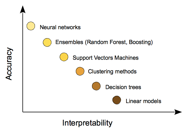
3. Trade-off between Accuracy and Interpretability
The thing is that not all kinds of machine learning models are equally interpretable. As a rule, more accurate and advanced algorithms, e.g. neural networks, are hard to explain. Imagine making sense of all these layers' weights!
Thus, it is a job of a data scientist to:
- Find a trade-off between accuracy and interpretability.
- Explain a choice of a particular algorithm to a client.
One may use a linear regression which predictions are easy to explain. But the price for a high interpretability may be a lower metric as compared to a more complicated boosting.
4. Feature importance
Feature importance helps to answer the question "What features affect the model's prediction?"
One of the methods used to estimate the importance of features is Permutation importance.
Idea: if we permute the values of an important feature, the data won't reflect the real world anymore and the accuracy of the model will go down.
The method work as follows:
- Train the model
- Mix up all values of the feature X. Make a prediction on an updated data.
- Compute $Importance(X) = Accuracy_{actual} − Accuracy_{permutated}$.
- Restore the actual order of the feature's values. Repeat steps 2-3 with a next feature.
Advantages:
- Concise global explanation of the model's behaviour.
- Easy to interpret.
- No need to re-train a model again and again.
Disadvantages:
- Need the ground truth values for the target.
- Connection to a model's error. It's not always bad, simply not something we need in some cases.
Sometimes we want to know how much the prediction will change depending on the feature's value without taking into account how much the metric will change.
5. Dependency plots
Partial Dependency Plots will help you to answer the question "How does the feature affect the predictions?" PDP provides a quick look on the global relationship between the feature and the prediction. The plot below shows that the more money is at one's bank account, the higher the probability of one signing a term deposit during a bank campaign.
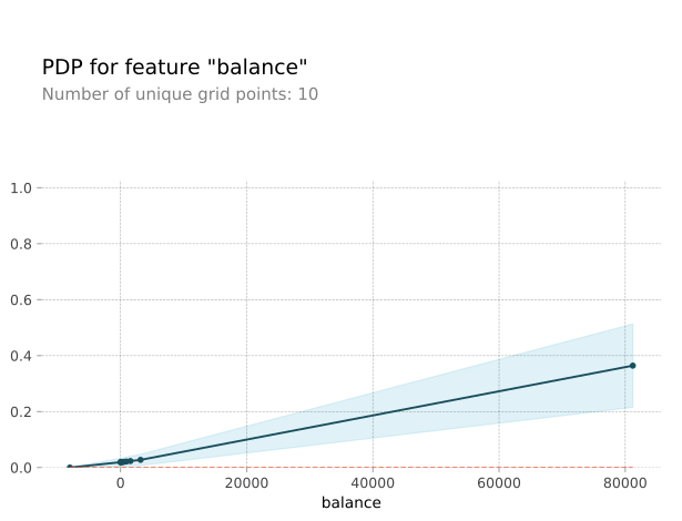
Let's look at how this plot is created:
- Take one sample: a single student, no loans, balance is around $1000.
- Increase the latter feature up to 5000.
- Make a prediction on an updated sample.
- What is the model output if balance==10? And so on.
- Moving along the x axis, from smaller to larger values, plot the resulting predictions on the y axis.
Now, we considered only one sample. To create a PDP, we need to repeat this procedure for all the samples, i.e. all the rows in our dataset, and then draw the average prediction.
Advantages:
- Easy to interpret.
- Enables the interpretation of causality
Disadvantages:
- One plot can give you the analysis of only one or two features. Plots with more features would be difficult for humans to comprehend.
- An assumption of the independent features. However, this assumption is often violated in real life. Why is this a problem? Imagine that we want to draw a PDP for the data with correlated features. While we change the values of one feature, the values of the related feature stay the same. As a result, we can get unrealistic data points. For instance, we are interested in the feature Weight, but the dataset also contains such a feature as Height. As we change the value of Weight, the value of Height is fixed so we can end up having a sample with Weight==200 kg and Height==150 cm.
- Opposite effects can cancel out the feature's impact. Imagine that a half of the values of a particular feature is positively correlated with the target: the higher the value, the higher the model's outcome. On the other hand, a half of the values is negatively correlated with the target: the lower the feature's value, the higher the prediction. In this case, a PDP may be a horizontal line since the positive effects got cancelled out by the negative ones.
6. Local interpretation
For now, we have considered two methods of global interpretation: feature importance and dependecy plots. These approaches help us to explain our model's behaviour, well, at a global level which is surely nice. However, we often need to explain a particular prediction for an individual sample. To achieve this goal, we may turn to local interpretation. One technique that can be used here is LIME, Local Interpretable Model-agnostic Explanations.
The idea is as follows: instead of interpreting predictions of the black box we have at hand, we create a local surrogate model which is interpretable by its nature (e.g. a linear regression or a decision tree), use it to predict on an interesting data point and finally explain the prediction.
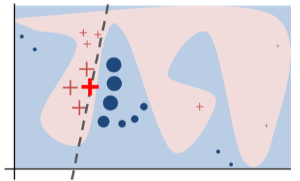
On the picture above, the prediction to explain is a big red cross. Blue and pink areas represent the complex decision function of the black box model. Surely, this cannot be approximated by a linear model. However, as we see, the dashed line that represents the learned explanation is locally faithful.
Source: Why Should I Trust You?
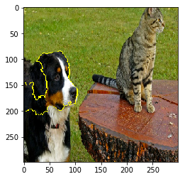
Here is the example of local interpretations for classifications of animals on an image.
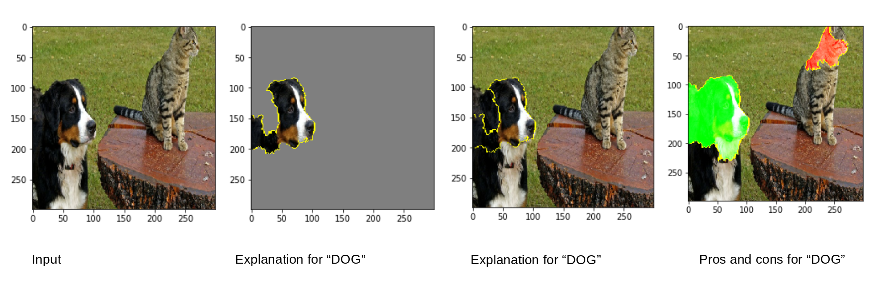
Source: LIME Tutorial
Advantages:
- Concise and clear explanations.
- Compatible with most of data types: texts, images, tabular data.
- The speed of computation as we focus on one sample at a time.
Disadvantages:
- Only linear models are used to approximate the model's local behaviour.
- No global explanations.
7. SHAP
SHapley Additive exPlantions (SHAP) is an method based on the concept of the Shapley values from the game theory.
Idea: a feature is a "player", a prediction is a "gain". Then the Shapley value is the contribution of a feature averaged over all possible combinations of a "team".
Advantages:
- Global and local interpretation.
- Intuitively clear local explanations: the prediction is represented as a game outcome where the features are the team players.
Disadvantages:
- Shap returns only one value for each feature, not an interpretable model as LIME does.
- Slow when creating a global interpretation.
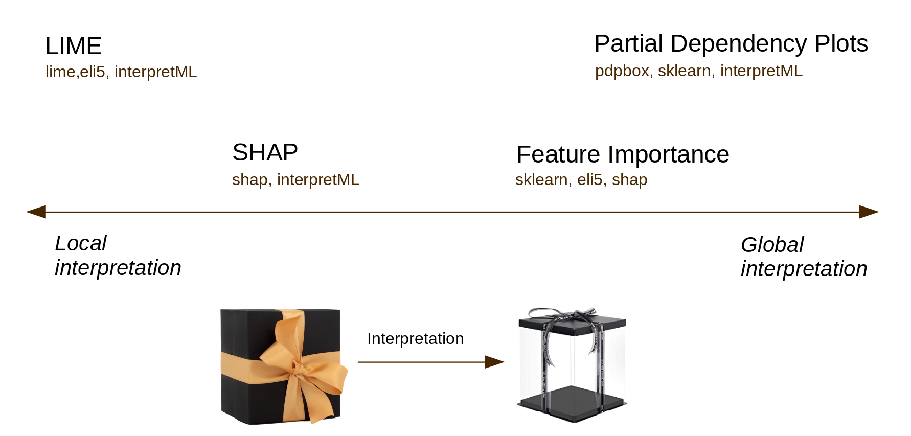
P.S. A quick (but totally not comprehensive!) overview of some tools for interpretable ML.